We first introduce components of our program (and their informal meanings)
means a command that does nothing.
A variable
is a string or a name. The set of all variables is denoted by
.
Definition 1.1 (Syntax of Arithmetic Expression).The syntax of arithmetic expressions is
defined as
where stands for
integer division,
stands for mod. We add parentheses here to avoid the arithmetic priority issue, and will omit them
later on.
The set of all arithmetic expressions is denoted by
.
Definition 1.2 (Syntax of Boolean Expression).The syntax of a boolean expression is defined
as
where
is an arithmetic expression.
The set of all arithmetic expressions is denoted by
.
Then we can define the syntax of program.
Definition 1.3 (Syntax of Program).The syntax of a program
is
defined as
where ,
is an
expression, and
means a sequence of two program.
The meaning of these programs are not formally defined yet. We will add more program syntax
later.
1.2 Semantics of Expressions
Definition 1.4 (Valuation).A valuation is a function ,
which specifies values of variables. The set of all valuations is denoted by .
Given a valuation ,
the value of the variable
is .
During the execution of the program, the variable itself remains the same (just a name), but
its value changes as the valuation changes.
Definition 1.5 (Semantics of Arithmetic Expression).The semantics of an expression
is the meaning / value of the expression, denoted by .
Formally,
is a function
(not ),
such that the value of function
at ,
denoted by
or simply ,
is the value of expression
given the valuation .
We can immediately get the semantics of some simple expressions by definition:
,
.
.
,
similar for .
Definition 1.6 (Semantics of Boolean Expression).The semantics of a Boolean expression
is a function ,
such that
is the truth value of
given a valuation .
For simplicity, we assume that non-zero numbers stand for
and zero
stands for ,
so that we do not need to explicitly name a domain for values of boolean variable.
Notation 1 (Inference-rule notation).
means that if the Assumptions are true, then the Result is true.
Semantics of more complex expressions can be defined as rules under some assumptions:
:
.
:
.
:
,
similar for .
:
.
:
.
Rules for boolean expressions:
Assume that
stands for false and nonzero stands for true.
.
:
,
similar for other comparison operations.
:
.
By shortcircuiting with the first condition, we use one less rule. Similar for or.
1.3 States
Definition 1.7 (State of Program).We can define the state of a program as:
1.
The current valuation: .
2.
The current valuation together with a pointer showing the current position in code:
where
is a line number.
3.
The current valuation together with a piece of remaining code to be executed: .
We denote by
the set of all states. Program execution is simply captured by transitions between states.
Analysis of the 3 types of states:
1.
The first type :
Doesn’t tell the intermediate process of the program (terminations, exceptions).
2.
The second type :
E.g.,
      while x > 0 && y > 0 do
        if x > y then
          x = x - y
        else
          y = y - x
        fi
      od
Suppose the initial valuation is
for
respectively. Then the execution process can be represented as
.
Drawbacks: Requires knowing the whole program, cannot model separate functions in the
program independently.
3.
Thus, we use the third type of state .
E.g., x = 1; y = x + 2 can be represented as
.
1.4 Operational Semantics
Definition 1.8 (Operational Semantics).Operational semantics is a category of semantics
that is defined by inference rules over transitions between states.
1.4.1 Small-Step (Structural) Semantics
Definition 1.9 (Small-step Transition Relation).A samll-step transition relation
means that the first state transits to the second state in one execution step.
where
means an empty program. We sometimes abbreviate
to
.
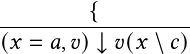
Assignment:
where means the
same valuation as
except that
is set to ,
i.e.,
and .
Halt:
means that the execution ends immediately.
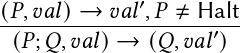
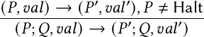
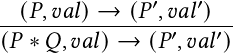
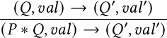
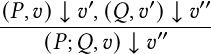
Sequential composition:
.
If the case is not excluded,
the result would be ,
meaning that it does not terminate and will continue to execute
.
If-else:
,
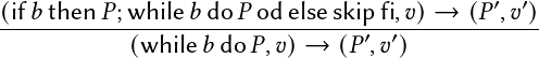
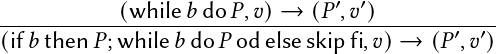
While loop:
,
Combining this with the inference rules for
,
we can derive the following corollaries:
,
also called the unrolling.
Non-determinism:
means that either
or
will be executed but the program does not know which one it is in advance. (E.g., controlled by
the user).
,
dependent on which one of
or is
executed.
Consider the extension with ,
, and
:
For: means that first
initialize with , then
as long as holds repeat
executing followed
by updating with .
That is
Then the semantics of
can be defined based on the sequential composition and
.
and
in
.
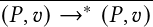
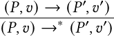
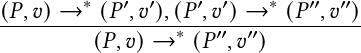
1.4.2 Transitive Closure
Definition 1.11 (Transitive closure).
means that starting from state ,
we can reach state
in certain number of steps. Formally, it is defined by
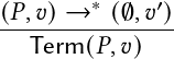
1.4.3 TODO Termination
Definition 1.12 (Termination).A program
with valuation
will terminate if it will eventually transit to an empty program, denoted by
.
Formally, it is defined by
.
E.g., prove the Euclidean Algorithm for calculating the GCD terminates
:
TODO We denote the program by ,
the condition in while by ,
and the body by .
Case 1: ,
Case 2: ,
similar.
Case 3:
and . Denote
(substitute
by
in the following, not
assigning in the beginning).
We prove by induction on :
Base case .
Omitted.
Induction step (programs
with the value of
less than the current value all terminate). We only prove the case where
initially, and the other situation is symmetric.
1.4.4 Big-Step Semantics
Definition 1.13 (Big-Step Relation).A big-step relation
means that the program
with valuation terminates, modifyng the valuation to .
and
are
equivalent only if (necessary but not sufficient),
This is not sufficient because the termination is not taken into consideration.
Example 1.1.Consider
and .
always terminates with ,
but
terminates only when sometimes
is executed. We could not say they are equivalent.
1.5 Denotational Semantics
Definition 1.15 (Denotational Semantics).Denotational semantics is a category
of semantics that is defined as mathematical functions. Usually, the denotational semantics of
a program is obtained inductively based on the (already defined) denotational semantics of its
subprograms.
We are going to use the current valuation for state, i.e., the set of state
.
The type of semantics of arithmetic / boolean expressions does not change (but
becomes
): If
is an arithmetic
expression, then .
If is a boolean
expression, then .
The denotational semantics of them basically rewrites the inference rules (operational semantics) as
operations on functions:
Base: ,
.
,
similar for other arithmetic expressions.
Base: ,
.
,
,
similar for other boolean expressions.
Definition 1.16 (Denotational Semantics of Program).The semantics of a program
is the function that transforms the initial state (valuation) to the final state (valuation), denoted
by .
Formally, it is a partial function .
It is partial because it is not defined on initial states that do not terminate, etc.
Definition 1.17 (Conditional statement).Let
, then the conditional
semantics
is defined as
E.g., we can rewrite
as .
Semantics of program (check that the R.H.S.s are valuations):
.
.
◦.
(Composition)
If:
(check that the types of the arguments conform to the definition).
Semantics of while:
Problematic: .
According to the semantics of sequential composition above,
is defined based on ,
which forms a cycle.
Recall that
should be equivalent to
(derived from the Operational Semantics).
In other words, we want to assign a function to
and consequently a function to
such that these two functions
are the same.
Given , we define
a transformer
as
◦
Plugging in
and unrolling ,
we have
◦
(in Denotational Semantics).
Thus, the requirement that the two functions are the same are met if and only if
(in Denotational Semantics). That is, if and only if
is a fixed
point of .
Two questions:
Does the fixed point exist for ?
Is the fixed point unique?
We will answer them next.
This way of defining the semantics does not involve the issue of cycle definition. Also, we do
not care about how to compute the fixed point, but only need to assign mathematical definition
to it.
Proposition 1.1.Given an boolean expression
and a program ,
there exists a fixed point of .
Proof 1.1.We prove by constructing functions based on Operational Semantics.
For any program
and valuation ,
we define
iff
in Operational Semantics, and
if there is no such
(does not terminate).
Running the inference rules, we will get a function
for
and a
function
for .
Recall the corollary about the equivalence between two, which basically means
Thus, .
is
indeed a fixed point.
Proposition 1.2.The fixed point is not unique, but the least defined fixed point is unique.
Proof 1.2.We can prove the nonuniqueness simply by finding multiple fixed points:
iff
◦
So could be
for any constant
function
().
Proof 1.3.More detailed analysis of constraints on the fixed points: Let
be any fixed
point of
(abbreviated to
below). Let
be an arbitraty initial valuation, then there are three possible cases of the while loop.
1.
The entire while loop terminates after a finite number, say ,
of iterations:
We have
for .
Moreover,
This implies that
◦◦
for ,
and .
Since
is a fixed point,
2.
Some iteration, say the -th
one, does not terminate so the whole loop does not terminate.
Equation (1) still holds for .
And we have
Then, equation (2) also holds for .
Since is a
fixed point of ,
3.
Every iteration terminates but the loop itself does not:
Equation (1) and
holds for .
Similarly, we have
Equations (*1), (*2), and (*3) are the only constraints we have on
in the three cases, respectively.
In (*1) 1, the values are
uniquely determined to be .
However, in (*2) and (*3), the values are not unique.
We want the
that aligns with the Operational Semantics. Requirements are:
Case 2:
since it does not terminate. Thus, ,
which should be .
Hence, .
Case 3:
since the while loop does not terminate. Thus, .
Now, this
is uniquely determined.
Least defined fixed point: A fixed point such that at any initial valuation it is not uniquely determined,
its value is .
The
uniquely determined above is the least defined fixed point.
1.5.1 Non-Determinism
Without non-determinism, .
Let ⟳ be the state representing
non-termination, so that ⟳.
More explicitly, ⟳, since no
valuation is mapped to .
With non-determinism, ⟳.
.
.
.
,
where
is also extended to ⟳.
For while, we also find a fixed point of the transformer, but the definition of the transformer is
more complicated.
1.6 Axiomatic Semantics and Hoare Logic
Definition 1.18 (Invariant).Assertion assigned to some point of the program that always
hold whenever the program reach the point.
E.g., the first line of a while loop may reached many times.
Definition 1.19 (Pre-conditon and post-conditon).The invariant that is assigned to the
beginning or the end of a (part of) program, respectively.
E.g.,
1.6.1 Hoare Triples
Definition 1.20 (Hoare triple).A hoare triple
, where
and
are two assertions and
is a program, means
that, for any current ,
if holds in
state (denoted
by ), and
is a state that can be reached
by a terminating run of
starting at ,
then holds
in state .
Formally,
is defined as the logical statement
⊧⊧
Remark: the assertion can be .
always holds
( holds)
and never
holds (
holds).
If the program does not terminate, the Hoare triple does not say anything.
Hoare triples talk about all possibilities of the program execution.
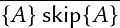
Axioms:
Skip axiom
Assignment axiom schema
where
means the same assertion except that every valuation at
is replaced by the
semantics of at
the valuation ().
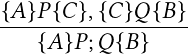
Sequential composition
If
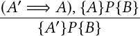
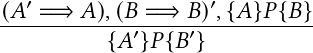
Consequence: Strengthen the pre-condition
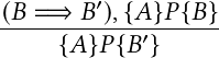
or weaken the post-condition
or both
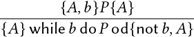
While:
is called the loop invariant (the invariant right before while)
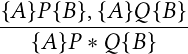
Non-determinism:
2 Infinite-duration Two-player Games on Graphs
2.1 Basic Concepts
Games in which two players play forever.
Definition 2.1.A game graph or arena is a finite directed graph
with a
partition
of ,
where
and
belong to the two players, respectively,
every vertex has at least one out-going edge.
Given an initial vertex ,
the game proceeds as follows:
At a vertex
player
transitions the state along of the out-edges of .
An outcome is an infinite (by 2.1) path resulting from the game play.
An objective for a player is a set of outcomes. The player wins if the outcome is in the
objective.
A game is zero-sum if the objective of one player is the complement of the objective of
the other player.
2.2 Classical Objectives
Let be an infinite path.
We denote the prefix of
starting from the -th
vertex by .
Define:
.
,
nodes visited infinitely many times by .
Let
be a subset of vertices, here are some of the classical objectives:
Definition 2.2.Let
be a set of target vertices. Then,
the (alternating) reachability objective is defined as ,
i.e., the set of outcomes that ever reach (some vertices of) .
The problem of finding the initial vertices from which player 1 can win is called the
(alternating) reachability game problem.
The safety objective is defined as ,
i.e., the set of outcomes that only traverse within .
Definition 2.3.Let
be a set of Büchi vertices. Then,
The Büchi objective is defined as ,
i.e., the set of outcomes that visit (some vertices of)
infinitely many times.
The coBüchi objective is defined as ,
i.e., the set of outcomes that visits vertices out of
only finitely many times (enter
at some time and then never leave ).
We can check that:
Definition 2.4.Let
be a priority function. Then the parity objective is defined as .
It is the most general objective we will study.
Proposition 2.1.
where
for
and
otherwise.
In this case, .
Proposition 2.2.
where
for
and
otherwise.
To find a priority function for coBuchi, we want
. This hints that we
set to be a smaller
odd number for .
Proposition 2.3.In general,
for
(or
for ).
Definition 2.5.We say an objective
is a tail objective if whenever ,
we have
for every .
Proposition 2.4.Parity objectives are tail objectives since finite prefix does not matter.
2.3 Strategy
Notation 2.For a vertex ,
we denote by
the set of successor vertices of .
Definition 2.6.A strategy for player
is a function ,
where
represents the history (the portion of path visited) domain. Given history
and current vertex
, the strategy outputs
Player ’s chioce of the
next vertex to visit .
is called memoryless if it is only based on the current state:
for all .
In this case, we can denote .
is called persistent if back to the same vertex it still makes the same decision:
for all paths
such that
is a prefix of ,
denoted by .
Notation 3.The outcome is fixed given the initial vertex
and strategies (no matter memoryless or not) of the two players .
We denote it by .
Without other specifications, we assume that strategies are memoryless in the following
discussion.
Remark 1.In the case where strategies have memory, one may discuss the size of the memory.
The memory is said to be finite if it has finite bits (not that it can memorize finite number of
steps).
Definition 2.7.A strategy
for player
is called a winning strategy for player 1 from a vertex
if for every strategy
of player
we have .
The winning strategies for player
are defined analogously.
Definition 2.8 (Spoiling strategy).A strategy
for player
spoils
if .
Definition 2.9.Given an objective
for player ,
the winning set
is the subset of vertices from which player
has a winning strategy (i.e., the other player has no spoiling strategy for this).
Definition 2.10.A game with objectives
for players 1 and 2 respectively is determined if .
Usually we aim at finding the winning set of player 1.
2.4 Solving Reachability Games
Suppose the objective for player 1 is .
(Besides attractors and traps for this objective, I also include some related conclusions on winning strategies for player
2 and objective .)
Definition 2.11.Let
be a set of target vertices. The attractor for player
is defined as ,
the set of vertices from which player
has a strategy to reach .
Proposition 2.5. The set
can be inductively defined as follows:
Base case
(trivial)
Inductive step: Assume
is a subset of the attractor. Consider some initial vertex
that is not yet included.
If
belongs to Player 1 and has an edge towards ,
then Player 1 can move the state along the and win.
If
belongs to Player 2 and has only edges towards ,
then Player 1 can win too.
Therefore, setting ,
is an extended subset of attractor. The process stops when
. Then,
.
The inductive definition for
can be analogous.
Definition 2.12.For all vertices in ,
define
if
(See Prop. 2.5).
Proposition 2.6.By definition,
and .
[TODO: We will soon see that they are equal]
. Intuitively, consists of all
vertices that can reach in at most
steps, so any valid attractor
must be included in some .
Definition 2.13.Let be a set
of target vertices. A vertex set
is said to be trap for player 1 if player 2 has a strategy to confine the state in
(and hence
never reaches ),
i.e.,
1.
If ,
then
2.
If ,
then .
We often use the term “a trap of player 1 in ”
or “a trap of player 1 out of ”.
That is,
and .
Proposition 2.7.
is a trap for player 1.
Proof 2.1.
1.
.
2.
Suppose .
If ,
i.e., ,
then
for some .
In this case,
should have been added into ,
which is a contradiction. Thus, .
3.
Suppose .
If ,
i.e., ,
then we can partition
to several sets such that each set
for some .
should have been added into ,
which is a contradiction. Thus, .
Derivation 2.1.Together, we have ,
and .
This implies that
Proposition 2.8.
and .
Find
using a BFS:
_______________________________________________________________________________________
Algorithm 1: Linear Algorithm for Finding Attractor___________________________________________________________ Input: Game
graph
,
set
of
target
vertices
Output: Attractor
set
1;
2;
3for
all;
4whiledo567Pop
one
vertex
from
;
8;
9fordo101112;
13ifthen1415
// Corresponds
to16;
17ifandthen1819
// Corresponds
to20;
21return;
Running time:
Visits all vertices: .
Visits all in-edges of :
.
Overall: .
2.5 Solving Buchi Games
Consider the zero-sum Buchi game with
and . We want
to solve
and .
Definition 2.14 (Subgame arena).Given an arena
and a set ,
if every vertex in
has a successor in ,
then the subgame arena at
is defined as
(remain edges within
only).
The condition of having a successor is to ensure that the
satisfies the third requirement of arena, which is every vertex has at least one out-going
edge.
We denote .
may not have a subgame arena: For m
,
it must have an edge to .
However,
may not satisfy the conditoin.
has a subgame arena iff every vertex in
has a successor in .
Any trap has a subgame arena: Check the definition. In particular,
has a subgame arena.
has a subgame graph: The base case is a trap ,
and hence satisfies the condition.
Since
is a trap for player 2, it also has a subgame arena.
2.5.1 Classical
Algorithm
Proposition 2.9.Player 2 has a winning strategy (for )
starting from ,
and hence player 1 does not have a winning strategy from the set. ().
Proof 2.2.
Player 2 first plays the strategy that reaches .
During this process, the path can only reach
finitely many times.
Then play the strategy that stays in .
Since ,
the outcome visits
only finitely many times.
Proposition 2.10.The following algorithm finds
and :
Mark all vertices in
as winning for Player 2, and recursively solve the subgame at
with objective .
Formally:
_______________________________________________________________________________________
Algorithm 2: Classical Algorithm for Finding coBüchi Winning Set__________________________________ Input: Game
graph
,
target
set
Output: Winning
set
1;
2fortodo345;
6;
7;
8;
9;
10;
11;
12ifthen131415break;
16return;
and
.
Proof 2.3.We first show that, in each iteration, it is “safe” to keep the subgame at
only (subscript omitted),
i.e., the game starting from
will remain in
if both players play the best. (Note that this does not include edges acrossand either). Consider
any initial vertex in :
Since player 2 can definitely win in ,
player 1 wants to avoid entering .
is a trap for player 2, so player 1 does have a strategy to keep the game in .
Also,
induces a subgame arena.
Then we show that player 1 has a winning strategy in
. Suppose the
loop breaks at ,
i.e., . The
must
be ,
since .
Thus, .
Then,
playes two roles:
It is a trap :
Recall from the beginning of this proof, the game will remain in
starting from .
It is the attractor : Player
1 has a strategy to reach
(not only in ,
but also in the entire graph). The state either:
is in ,
player 1 play the strategy to reach ,
or stays in
for a while and then enter
again.
So player 1 has a winning strategy (for )
and player 2 does not (for ).
Corollary 2.1.Buchi game is determined,
():
Corollary 2.2.Both winning strategies for player 1 and player 2 are memoryless: Their
strategies can be decomposed into many stages of reachability strategies, which are
memoryless.
Runtime of the algorithm: (attractor
algorithm) for each iteration. At most
iteration. Overall .
Solving :
. Solve
using
the algorithm.
2.5.2 Faster
Algorithm
More detailed analysis of the classical algorithm:
The running time for set operations on vertices sums up to .
Proposition 2.11.The total running time for finding all
(and removing relevant vertices and edges to derive )
is .
Proof 2.4.In the process of finding ,
all the vertices in
and their in-edges are visited.
Then it removes all edges incident on these vertices, i.e., all in-edges and out-edges.
Thus, every edge is visited
times.
The bottleneck is .
Notice that the only property of we
use is that it is a trap of player 1 out of .
We took as the largest such
trap, namely , but actually
it can be any trap out of .
Definition 2.15 (Subgraph Trap).Let ,
a set is an
-trap of player
1 outside if
For every ,
there is an outgoing edge
with
For every ,
for every outgoing edge ,
and .
It is a set of vertices from which player 2 has a strategy to restrict the state in the set and in the subgraph
when playing in the entire arena. It is not the same as a trap of player 1 outside
when playing in the
subgame arena .
We can use an algorithm similar to the reachability algorithm to find the maximum
-trap:
_______________________________________________________________________________________
Algorithm 3: Linear Algorithm for Finding Subgraph Trap_________________________________________________ Input: Game
graph
,
subgraph
,
and
target
set
Output: Trap
set
1
; // Change2;
3for
all;
4whiledo567Pop
one
vertex
from
;
8;
9fordo1011
// Change12;
13ifthen141516;
17ifandthen181920;
21;
22return;
It is basically the complement of the
“-attractor”
to the union of
and player 1-vertices which have an outgoing edges not in
.
Again, we cannot simply apply the previous algorithm to the subgame
.
Hierarchical Decomposition:
Order the edges in
such that edges
with
are prior to others.
Define the graphs
as follows:
where includes
the edge
if and only if at least one of the followings holds:
Out degree of
in
is ,
is one of the first
in-edges of
(w.r.t. the order defined above)
Every vertex in
has at most
out-edges and
in-edges in ,
so has at
most
edges.
The last subgraph is just the original graph.
Coloring Vertices:
Low-degree vertices, i.e. those with an outdegree of at most
in ,
are colored white.
High-degree vertices, i.e. those with an outdegree of more than
in ,
are colored blue if they belong to player 1 or colored red if they belong to player 2.
Proposition 2.12.Let
be the set of vertices that are
either blue in
or red in
with no outgoing edges in .
Then
is the set of all the vertices from which player 1 has a strategy to leave
(visit edges that
are not in ).
Proof 2.5.
White vertices in
have all its out-edges in
Red vertices in
with some out-edge in :
Player 2 can choose the edge to remain in .
Type-1 vertices in :
must have some out-edge not included in ,
so player 1 can choose the edge to leave.
Type-2 vertices in :
must have all outgoing edges outside ,
so player 2 has no choice but leave.
Proposition 2.13.The following algorithm finds a trap of player 1 outside of .
In addition, let
be the size of the found trap, then the algorithm takes
time:
_______________________________________________________________________________________
Algorithm 4: Algorithm for Finding Trap______________________________________________________________________________ Input: Game
graph
,
target
set
Output: Trap
for
player
1,
or
report
no
trap
found
1fortodo23
// Try
to
find
an-trapfor
player
1
out
of4Try
to
find
an
-trap
for
player
1
out
of
;
5ifsuchis
foundthen678Output
as
the
trap;
9break;
10ifno
trap
has
been
foundthen111213Report
no
trap
is
found;_______________________________________________________________________________________________________________________________
Proof 2.6 (Correctness).By definition, an -trap
of player 1 is an -trap
of player 1.
Proof 2.7 (Running Time).Suppose we find a trap
in the
-th iteration.
We claim .
We prove by casework on the color of player 1 vertices in the previous graph:
Case 1: There is a player 1 vertex
that used to be blue in .
Then
has an outdegree more than
in .
By definition, all the successors of
should be in the trap.
So the size of the trap is at least .
Case 2: All player 1 vertices in
used to be white in .
Then for every player 1 vertex in ,
all of its outgoing edges are in
and .
Then we claim that there exists a player 2 vertex
and another ,
such that the edge
is present in
in but not in .
If is is not the case, i.e., for every player 2 vertex
and every vertex in ,
if there is an edge between them, then the edge is also in .
Then we can check that the conditions for the presense of a -trap
are met, which is a contradiction.
Consider the predecessors of :
Since
is new in ,
it must be ranked between
to
among all in-edges of .
Since
is in a trap, .
Thus,
such that
is prior to ,
must also be in .
These predecessors belong to player 2 and have an edge to ,
so they are included in (the largest possible) trap .
So the size of the trap is at least .
In summary, the algorithm finds a trap of size
in
time. In other words, it
can find a trap of size
in
( is the
size of the actual trap it found).
The faster algorithm:
_______________________________________________________________________________________
Algorithm 5: Classical Algorithm for Finding coBüchi Winning Set__________________________________ Input: Game
graph
,
target
set
Output: Winning
set
1;
2fortodo345;
6
a
trap
of
size
computed
by
the
hierarchical
decomposition
algorithm;
7;
8;
9;
10;
11ifthen121314break;
15return;
Running time: Since
is removed from ,
all ’s add up to
, the overall
running time is .
2.6 Solving Parity Games
Consider a zero-sum game with
and ,
where .
W.l.o.g., we can assume that
either 0 or 1 appears in the priorities: If not, can shift all priorities to the left by 2.
priorities are contiguous: If not, we can shift any priority to the left by some multiple of
2 as long as it does not become less than the previous priority. More explicitly,
if the two adjacent priorities differ by some multiple of 2, then we can merge the
larger one into the smaller one,
if the two adjacent priorities differ by some multiple of 2 plus 1, then we can shift
the larger one to become the smaller one plus 1.
When there are more than two priorities, w.l.o.g., priority 0 appears in the game, because we can
solve .
Proposition 2.14.Parity game is determined and both players have memoryless winning
strategies.
Proof 2.8.We prove by induction on the number of priorities .
Base cases:
If there is only one priority, then the game is determined and the strategies do not matter.
If there are only two priorities, then the parity game is either a Buchi game ()
or a coBuchi game ().
Induction step: Assume any parity game with
priorities
is memoryless and determined. We want to show that any game with
priorities
is
memoryless and determiend by diminishing priority 0 in the current game.
1.
Firstly, we find :
Let .
Let
and
(trap of player 1 out of ).
has a subgame and the subgame does not have any priority 0 vertex. By induction,
the subgame with the same objectives is determined and memoryless. Let
be the winning sets of player 1 and 2, respectively, in the subgame at .
Player 2 has a winning strategy in the original game from :
Play the strategy that traps the game in
and the same winning strategy as in the subgame.
Player 2 has a winning strategy in the original game from :
First play the strategy that reaches
in finitely many steps, then play the above strategy. The finitely many steps does
not affect the parity (See Tail Objective).
The winning strategies above are memoryless.
Mark all vertices in
as winning starting vertices for player 2. And continue recursively on the subgame
at .
The argument is exactly the same as Buchi games.
2.
Secondly, we show that .
The process continues until .
We use the same notation for .
Consider this strategy for player 1: if the current state is in
,
then play the winning strategy as in the subgame; if the current state is in
,
then play the winning strategy for objective
.
Then no matter what strategy player 2 plays, player 1 can always win:
By definition, if player 2 keeps the game in ,
player 2 will loss and player 1 will win (determinanc in ).
Since the objective is a tail objective, if player 2 keeps the game in
after finitely many steps, player 2 will still loss and player 1 will win (determined
in ).
Otherwise, player 2 does not keep the game in
for infinitely many time, i.e., the game enters
for infinitely many times. Everytime the game is in ,
player 1 play with strategy for objective .
Thus, player 1 can reach priority 0 for infinitely many times. In this case, player
1 still win.
3.
This shows that the game is determined and memoryless.
Running time:
:
There are
iterations, each of which needs to solve a parity game with
priorities and finds attractors.
Base case:
(Buchi).
.
3 Automata on Finite Words
Definition 3.1 (Deterministic Finite Automaton, DFA).A Deterministic Finite Automaton (DFA) is
a tuple
in which:
is a finite alphabet of letters.
is a finite set of states.
is the initial state.
is the transition function.
is the set of accepting states.
A DFA operates on fintie words as follows: It starts from the initial state. Each each
symbol from the alphabet is read sequentially. If the current state and symbol are
and
respectively,
it transits to .
A word is accepted if the (unique) run with that word ends in an accepting state. (P.S. if the
transition corresponding to the input symbol is not available at the current state, then it directly
leads to a rejection.)
The language of the automaton is the set of accepted words.
P.S., we denote the set of all finite words consisting of letters in
by
.
Definition 3.2 (Nondeterministic Finite Automaton, NFA).A Nondeterministic Finite Automaton NFA
is a tuple
in which:
is a finite alphabet of letters
is a finite set of states
is the set of initial states
is the transition function (changed, can transit to multiple states)
is the set of accepting states
A word is accepted if there exists a run over the word ending in an accepting state.
3.1 Basic Closure Properties
Proposition 3.1.Any NFA has a NFA complement.
4 Automata on Infinite Words
(-automata)
We denote the set of all infinite words consisting of letters in
by
.
Definition 4.1 (Deterministic Automaton of Infinite Words).A Deterministic Automaton on Infinite
words is a tuple
in which:
is a finite alphabet of letters.
is a finite set of states
is the initial state
is the transition function
is an acceptance condition formalizing when a run is acepting.
Definition 4.2 (Nondeterministic Automaton on Infinite Words).A Nondeterministic Automaton on Infinite
words is a tuple
in which:
is a finite alphabet of letters.
is a finite set of states
is the initial state
is the transition function
is an acceptance condition formalizing when a run is acepting.
The Automata on Infinite words with the acceptance condition being Buchi or Parity are called
Buchi Automata and Parity Automata, resp.
4.1 Buchi Automata
Definition 4.3 (Buchi Automaton).A Buchi Automaton is an Automaton on Infinite words
with Buchi acceptance condition: Let
be the target set, a run
is accepting if it visits T infinitely many times, i.e. .
We abbreviate Deterministics Buchi Automaton to DBW, and the nondeterministic one to
NBW.
Definition 4.4 (-regular Language).We call a language -regular
if it is the language of some NBW.
Proposition 4.1.NBW are strictly more expressive than DBW:
There is a language such that it is the language of some NBW, but is not language of any
DBW.
For any language, if it is the language of some DBW, then it must be the language of
some NBW.
Proof 4.1.The second statement is trivial: we can make a DBW NBW by turning the initial
state and the outputs of the transition function into sets of single element.
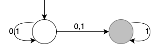
The first statement is proved by contradiction: Consider this NBW which accepts all words with
finitely many zeros (grey nodes are target states):
Suppose is a DBW with
the same language. Let
be the number of states in
(finite). Consider the following accepting infinite words:
11…1…, all ones: Let the first accepting state in the run be .
11…101…, same as the previous one except that a 0 is inserted right after :
Let the first accepting state after the 0 be .
and so on, the word with
0s and the -th
0 inserted right after :
Let the first accepting state after the -th
0 be .
By Pigeon principle, two among these accepting states, say
and
, must be the same. Let the
prefix of the last word before
be , and the
subsequence between
and (excluded)
be . Starting
from , the run of
returns to this state
by reading . Then
, the concatenation
of and infinite
repetitions of ,
is also accepted, because it visits accepting states infinitely many times.
However,
contains infinitely many zeros. This contradicts with the assumption. Thus, DBW with the same
language does not exist.
4.1.1 Complementation of DBW
In the followings, we will call languages that can be recognized by some DBW “DBW
languages”.
Proposition 4.2.DBW languages are not closed under complementation. There is some
DBW, such that we cannot find another DBW whose language is the complement of the
language of the first DBW.
Proof 4.2.Consider the example in the last proof: We showed that there is no DBW of the language
consisting of words with finitely many zeros. However, there exists a DBW of the language
consisting of all words with infinitely many zeros:
4.1.2 Union of DBWs
Proposition 4.3.DBW languages are closed under union. For any two DBWs, there is another
DBW that recognize the union of languages of the two DBWs.
Proof 4.3.Let
be any two languages. Suppose ,
where
and .
Consider the automaton that simulates the transitions of
at the same time: ,
where .
Each state of
is a pair of states of .
Then
accepts a word iff the run with the word visits
infinitely many times, which is equivalent to visiting
infinitely often, or visiting
infinitely often, or visiting both infinitely often. This means that the word is in .
Thus, .
4.1.3 Intersection of DBWs
Proposition 4.4.DBW languages are closed under intersection. For any two DBWs, there is
another DBW that recognize the intersection of languages of the two DBWs.
Proof 4.4.Let
be two automata and .
The tuples of
use the same notation as above.
consists of the words that visit both target sets infinitely many times, which is equivalent to
alternating between both target sets infinitely many times (before switching to the other
target set, can visit the same target set multiple times).
Consider two copies of the “joint” automata
.
We want to modify the transitions such that once the run reaches a target state in
one copy, it switches to the other copt and continue the transition, so that it cannot
visits target states in the same copy consecutively. We define the target set to be
and
by:
A run in visits
infinitely often iff
it visits infinitely
often: Once it visits ,
it switches to , and
visits zero or more
times until it visits .
vice versa.
4.1.4 Union of NBWs.
Proposition 4.5.-regular
languages are closed under union. For any two NBWs, there is an NBW that recognize the
union of languages of the two NBWs.
Proof 4.5.Let
and
and
be their languages, resp. We define ,
where .
Basically, we keep two isolated components in .
Then every accepting word in
corresponds to an accepting word in
starting from ,
and vice versa.
P.S.: Since DBW can have only one initial state, we cannot use this construction to prove the union of
two DBWs.
4.1.5 Intersection of NBWs
Proposition 4.6.-regular
languages are closed under intersection. For any two NBWs, there is an NBW that recognize
the intersection of languages of the two NBWs.
Proof 4.6.The same proof as DBW works. The initial set becomes .
The definition for
becomes
if ,
etc.
4.1.6 NBW Complement of DBW
Proposition 4.7.For any DBW, there is an NBW that recognize the complement of the
language of the DBW.
Proof 4.7.Let
be a DBW. Intuitively, in a complement NBW
with the “same” (not exactly) set of states as ,
the accepting words should never see
after finitely many steps.
We define
as follows: ,
i.e.,
plus an extra copy of .
.
.
,
.
The accepting words of
are not accepted by :
They visit
infinitely many times, and will never visit
(corresponds to
in )
once entering .
Conversely, the accepting words of
are not accepted by :
To visit
(
in )
infinitely often, they cannot ever enter .
Remark: This method is not applicable for finding NBW complement of NBW. In
the nondeterministic setting, an accepting words may have one run that visits
infinitely often and
another run that visits
infinitely often.
4.1.7 Emptiness of DBW/NBW
Given a DBW/NBW
with states,
decide whether .
iff there exists an
accepting run of with an
infinite word: Any valid run of
corresponds to a unique word, so the problem is equivalent to deciding whether
has an
accepting run.
Proposition 4.8.We can find a corresponding Buchi-game for emptiness problem: Let
be the set of accepting states in .
We call the graph
defined below the underlying graph of :
,
and
iff
(since we only care about the existence of an accepting run, not the characters in the run).
Define a single-player game ,
where
and ,
with objective .
Then
iff there exists an outcome starting from an initial vertex ,
which is equivalent to .
Proof 4.8.A run corresponds to an outcome, and an accepting run, which visits
infinitely often, corresponds to a winning outcome starting from an initial vertex in the game.
Since the outcome is solely controlled by player 1, the condition is equivalent to .
Thus, this is solvable using the algorithm for finding winning set of Buchi game in
or
time.
1.
Linear-time algorithm
Proposition 4.9.Consider the underlying game graph. Since the there are finitely many
vertices, a run visits
infinitely often iff it visits a particular vertex in
infinitely often. Furthermore, this is equivalent to that there (1) there is a cycle containing
a vertex in ,
(2) the cycle is reachable from the initial vertices.
Consider the strongly connected components of the graph. Condition (1) is equivalent to that
an accepting state is contained by some non-transitional SCC, which is a SCC that is not a
single vertex without a self-loop, i.e., a SCC that either is a single vertex with a self-loop or has
at least two vertices.
The algorithm:
(a)
Find all reachable vertices: Linear time.
(b)
Find all SCCs: Linear time (tarjan).
(c)
Check if a SCC contains an accepting state and is reachable: Linear time.
Overall, it is solvable in linear time .
4.1.8 Universality Problem of DBW
The dual of emptiness.
Given a DBW ,
decide whether .
For a DBW, every word has a unique run and vice versa. Thus,
iff every
run of
is accepting.
Proposition 4.10.We have a corresponding coBuchi game for universality problem: Let
be the set of accepting states in .
Define a game with the underlying graph of
as in the emptiness problem with objective .
Then, every run is accepting iff every path starting from an initial vertex is in ,
i.e., .
Thus, the problem is solvable using the algorithm for find winning set of coBuchi game in
or
.
1.
Linear-time algorithm
Proposition 4.11.
iff every reachable cycle in the graph contains an accepting state.
Proof 4.9.Otherwise, there is a path that repeats a cycle containing no accepting state
infinitely many times, and hence does not visit
infinitely many.
Every cycle contains an accepting state iff, after the removal of all accepting vertices, no cycle
exists: This can be checked easily.
The algorithm:
(a)
Remove all the unreachable vertices: Linear time.
(b)
Remove all the accepting vertices: Linear time.
(c)
Check whether there is a cycle in the remaining graph: Linear time.
Overall, it is solvable in linear time .
4.1.9 Universality Problem of NBW
Proposition 4.12.Non-universality of NBW is NP-hard.
Definition 4.5 (3-coloring Problem).Given a (undirected) graph ,
is it possible to color the vertices in
with 3 colors such that no two adjacent vertices have the same color?
Proof 4.10.We provide a reduction from 3-coloring, which is a classic NP-complete problem.
Given a (undirected) graph ,
let .
We create the following NBWs:
1.
The first NBW
is defined to accept all words that, when ignoring the colors, are not valid paths in
.
That is, a word
is accepting iff
is an invalid path in .
with Buchi condition, where:
A word is accepted by iff the
run ever transits through
for some .
Thus, the path associated with every accepting word contains an edge that is not in
,
and hence is invalid.
2.
The second NBW
is defined to accept all words in which there is a vertex that appears with two different
colors.
with Buchi
condition, where ,
,
and
An accepting word is of the form .
3.
The third NBW
is defined to accept all words that do not contain all edges of the graph. It is rather complicated to
define
in expression, so we only show a subpart of it: The initial vertex
includes
for all undirected
edges . The subpart
for an edge
is:
which accpets all the words that at least miss the edge
(in either direction).
4.
The fourth NBW
is defined to accepts all the words that have the same color twice in a row.
5.
The NBW
().
We claim that is
universal iff is not
3-colorable, i.e., is
not universal iff
is 3-colorable.
Only if side:
does not accept a word iff the word (a) is a valid path in
,
(b) assigns a unique color to each vertex, (c) visits all edges of
, and
(d) does not have the same color in a row. This is equivalent to that the word represent a valid
3-coloring of the graph.
If side: If
has a valid 3-coloring, then any infinite path that visits all edges together is an infinite word that is not
accepted by .
Corollary 4.1.Unless P=NP, there is no polynomial-time complementation of NBW.
Otherwise, we can run this polynomial-time complementation, and apply the (polynomial)
emptiness algorithm to the complement to solve the universality in polynomial time.
4.1.10 Complementation NBW
Given a NBW ,
find an NBW
such that .
Proposition 4.13.If we color each edge of a 6-vertex graph with one red and blue, then there
must be a monochrome triangle.
Proof 4.11.Vertex 1 must have three edges of the same color, say blue. Consider the three
vertices connected with 1 by blue edges. There are two cases: (1) At least two of them are
connected by a blue edge, in which a blue triangle is formed. (2) All of them are connected by
red edges, in which a red triangle is formed.
Theorem 4.1 (Ramsey Theorem for Infinite Graphs).Consider a complete infinite graphwhere every edge is colored by one of colors. There is an infinite monochrome clique (complete subgraph induced by some vertices) in.
Proof 4.12.Let
be an arbitrary vertex. Since there are finitely many colors, there is a color
such that
has infinitely many neighbours with edge of color .
Let the set of these neighbours be .
Consider the infinite graph .
For the same reason, there exists a vertex
and a color
with the same properties. Continuing this process forever, we get three infinite sequences
,
,
.
Thus, there is a color
that appears infinitely many times in .
Let .
Clearly,
()
is an infinite monochrome clique.
Definition 4.6 (Equivalence class).Given an NBW
,
we define an equivalence relaion over all non-empty finite words as follows: For
, we say
if
For every pair of states ,
there exists a run of
from
to
over
iff there exists a run from
to
over .
For every pair of states ,
there exists a run of
from
to
over
that visits
iff there exists a run from
to
over
that visits .
Define a function
for each vertex
that maps
to and
. Then
iff
. Let
be the equivalence
class of function ,
i.e., .
Since we have finitely many such functions, we have finitely many equivalence classes.
Proposition 4.14.Every
is regular (recognized by some NFA).
Definition 4.7.We can find an NFA that recognizes exactly
:
For every pair of states ,
create an NFA
that accepts all words
such that there is a run of
over
from
to .
We can take
to be the same as
except that the initial state is
and the accepting state is .
Note that
is non-deterministic, so the word it accepts may have other runs.
For every pair of states ,
create an NFA
that accepts all words
such that there is a run of
over
from
to
passing through .
could just be the intersection of
and an NFA that is the same as
except that the initial state is
and the set of accepting states is .
Since any NFA has an NFA complement, there are
that accepts all words that does not have a run from
to
and
that accepts all words that does not have a run from
to
passing through .
Let the NFA that accepts
all finite words. For ,
if ,
then
is the NFA that recognizes .
Proposition 4.15.For every infinite word ,
there is a decomposition ,
where
are two equivalence classes of finite words. That is,
must be the concatenation of some finite word in
and infinitely many finite words in .
Proof 4.13.Let
be any infinite word, where each
is a symbol. We define .
Consider the infinite complete graph .
We view equivalence classes as colors, and color the edge
with the (unique)
that contains .
By the Ramsey theorem, there is a color
such that there is an infinite monochrome clique
in which edges are all colored .
Particularly,
all have color .
Thus,
can be decomposed as ,
implying that ,
where
is the class containing .
Proposition 4.16.Let
and
be equivalence classes. Either
or .
Proof 4.14.Let ,
where
and
are finite words. Suppose ,
then by the definition of equivalence class, we can replace
by any word in the same class without affecting the times the run visits .
Thus, the altered infinite words should also be .
Proposition 4.17.-regular
languages are closed under complementation. Any NBW has an NBW complement.
Proof 4.15 (Complementing NBW).There are finitely many ,
so there are finitely many sets .
We have an NBW for every :
Take the NFA for .
For each accepting state, create edges that the initial states have. The initial states and accepting
states for the NBW are the same as the NFA.
We have an NBW for every :
Take the NBW for
and the NFA for .
For each accepting state of the NFA, create edges that the initial states of the NBW have. The
initial states of the resulting NBW are the intial states of the NFA, and the accepting states of
the resulting NBW are the accepting states of the NBW for .
Then take the union of NBWs of all
that does not intersect with .
Since every infinite word is in some ,
all the words in
are included.
4.1.11 Containment Problem
Given two DBW/NBW
and , decide
whether .
Note that . If we can
find the complement NBW
of (such
that ),
find the intersection automaton, and then answer the emptiness problem.
4.2 Parity Automata
Definition 4.8 (Parity Automaton).A Parity Automaton is an Automaton on Infinite words with Parity acceptance condition: Let
be a priority function, a run
of the automaton is accepting if it satisfies the parity condition, i.e.
is even.
We abbreviate Deterministic Parity Automaton to DPW, and the nondeterministic one to
NPW.
 means that if the Assumptions are true, then the Result is true.
![------------
[[𝑐]](𝑣)= 𝑐](game1x.png) .
.
![[[𝑥]](𝑣)=--𝑣(𝑥)](game2x.png) .
.
![[[𝑎1]](𝑣)= 𝑎1,[[𝑎2]](𝑣)= 𝑎2
---[[𝑎--+ 𝑎-]](𝑣)=-𝑎-+-𝑎----
1 2 1 2](game3x.png) ,
similar for
,
similar for ![[[𝑎 ]](𝑣)= 𝑎 ,[[𝑎 ]](𝑣)= 𝑎 ,𝑎 ≠ 0,𝑎 = 𝑏 + 𝑐𝑎 ,0 ≤ 𝑏 < |𝑎 |
---1---------1----2--------2--2-----1--------2-----------2
[[𝑎1/𝑎2]](𝑣)= 𝑐](game4x.png) .
.
![[[𝑎1]](𝑣)=--𝑎1,[[𝑎2]](𝑣)=--𝑎2,𝑎2 >-0,𝑎1-=-𝑏 +-𝑐𝑎2,0-≤-𝑏-<-𝑎2
[[𝑎1%𝑎2]](𝑣)= 𝑏](game5x.png) .
.![-----------------
[[true]](𝑣)= true](game6x.png) .
.
![[[𝑏1]](𝑣)=--𝑎1,[[𝑏2]](𝑣)=--𝑎2,𝑎1->-𝑎2
[[𝑏1 > 𝑏2]](𝑣)= true](game7x.png) ,
similar for other comparison operations.
,
similar for other comparison operations.
![[[𝑏1]](𝑣)≠-0,[[𝑏2]](𝑣)≠--0
[[𝑏1and 𝑏2]](𝑣)= 1](game8x.png)
![--[[𝑏1]](𝑣)=-0--
[[𝑏1and 𝑏2]]= 0](game9x.png)
![[[𝑏1]](𝑣)-≠-0,[[𝑏2]](𝑣)=--0
[[𝑏1and 𝑏2]](𝑣)= 0](game10x.png)
![[[𝑒]](𝑣)= 𝑎
------------------------
(𝑥 = 𝑒,𝑣)→ (∅,𝑣[𝑥 \ 𝑎])](game12x.png)
![[[𝑏]](𝑣)= false
------------------------------
(if𝑏then 𝑃 else 𝑄fi,𝑣) → (𝑄,𝑣)](game17x.png)
![[[𝑏]](𝑣)= true
------------------------------
(if𝑏then 𝑃 else 𝑄fi,𝑣) → (𝑃,𝑣)](game18x.png)
![[[𝑏]](𝑣)= false
---------------------------
(while 𝑏do 𝑃 od,𝑣)→ (∅,𝑣)](game19x.png)
![[[𝑏]](𝑣)= true
-----------------------------------------
(while𝑏 do𝑃 od,𝑣) → (𝑃;while 𝑏do 𝑃 od,𝑣)](game20x.png)
![[[𝑏]]= true
------------------------------------------------------------------
(while 𝑏do 𝑃;Continue; 𝑄 od,𝑣)→ (𝑃;while 𝑏do 𝑃;Continue; 𝑄 od,𝑣)](game25x.png)
![------------[[𝑏]]=--true-------------
(while 𝑏do 𝑃;Break; 𝑄od, 𝑣)→ (𝑃,𝑣)](game26x.png)
![𝑣(𝑥) ≤ 0
------------
[[𝑥]](𝑣)-≤-0,[[0]](𝑣)=--0,0-≤-0
[[𝑥 >-0]](𝑣)=--false-
[[𝑔]](𝑣)= false
---------------
(𝑃,𝑣)-→-∗(∅,𝑣)-
(𝑃,𝑣)→---(∅,𝑣)-
Term( 𝑃,𝑣)](game31x.png)
![[[𝑛]](𝑣′)< [[𝑛]](𝑣)
-------------′-----
Term( 𝑃,𝑣 )](game32x.png) (programs
with the value of
(programs
with the value of ![-------′′-------omitted----------------
[[𝑛]](𝑣-)=--[[𝑥]](𝑣),[[𝑥]](𝑣)-<-[[𝑛]](𝑣)
[[𝑥]](𝑣)-≥-1,[[0]](𝑣)=-0,1->-0 ---symmetric------𝑥 >-𝑦,omitted-- [[𝑛]](𝑣′′)<-[[𝑛]](𝑣)-
[[𝑥 > 0]](𝑣) ≠ 0 ,[[𝑦 > 0]](𝑣)≠ 0 (𝑃′,𝑣)→ ∗ (∅,𝑣′′), (𝑃,𝑣 ′′)→ ∗ (∅,𝑣′)
---------------------------------------------- ----------′--------∗----′---------
[[𝑔]](𝑣)-≠-0-----------------,-------------------(𝑃-;𝑃,𝑣)→---(∅,𝑣-)
(if-𝑔then-𝑃;𝑃-else-skip)-→-∗-(∅,𝑣′)-
(𝑃,𝑣) → ∗ (∅, 𝑣′)
---Term(𝑃,-𝑣)---](game33x.png)
![[[𝑏]](𝑣)=-true,(𝑃,𝑣)-↓ 𝑣
(if𝑏 then 𝑃 else 𝑄,𝑣)↓ 𝑣′](game37x.png)
![′ ′ ′′
[[𝑏]](𝑣)=--true,(𝑃,-𝑣)↓-𝑣,(while-𝑏do-𝑃,𝑣-)↓-𝑣-
(while 𝑏do 𝑃,𝑣) ↓ 𝑣′′](game38x.png)
![----------------------
{𝐴[ 𝑥 \ [[𝑒]]]} 𝑥 = 𝑒{𝐴}](game40x.png)